This article produces a gallery of figures and tables produced by this package for reference.
library(cmfproperty)

ratios <-
  cmfproperty::reformat_data(
    data = cmfproperty::example_data,
    sale_col = "SALE_PRICE",
    assessment_col = "ASSESSED_VALUE",
    sale_year_col = "SALE_YEAR",
  )
#> [1] "Filtered out non-arm's length transactions"
#> [1] "Inflation adjusted to 2019"
stats <- cmfproperty::calc_iaao_stats(ratios)regression_tests
summary_info <-
cmfproperty::regression_tests(ratios, produce_table = TRUE)| Dependent Variable | |||
| ASSESSED_VALUE | log(ASSESSED_VALUE) | RATIO | |
| (1) | (2) | (3) | |
| SALE_PRICE | 0.77*** | -0.0000*** | |
| (0.001) | (0.00) | ||
| log(SALE_PRICE) | 0.91*** | ||
| (0.001) | |||
| Constant | 34,702.12*** | 0.95*** | 0.96*** |
| (256.32) | (0.01) | (0.001) | |
| Observations | 308,031 | 308,031 | 308,031 |
| R2 | 0.84 | 0.86 | 0.03 |
| Adjusted R2 | 0.84 | 0.86 | 0.03 |
| Note: | p<0.1; p<0.05; p<0.01 | ||
kableExtra::kable(summary_info)| Model | Value | Test | T Statistic | Conclusion | Model Description |
|---|---|---|---|---|---|
| paglin72 | 34702.1237052 | > 0 | 135.385620 | Regressive | AV ~ SP |
| cheng74 | 0.9136623 | < 1 | 1348.353690 | Regressive | ln(AV) ~ ln(SP) |
| IAAO78 | -0.0000001 | < 0 | -97.596795 | Regressive | RATIO ~ SP |
| kochin82 | 0.9359248 | < 1 | 1348.353690 | Regressive | ln(SP) ~ ln(AV) |
| bell84 | 20314.8672457 | > 0 | 77.266036 | Regressive | AV ~ SP + SP^2 |
| 0.0000000 | < 0 | -157.626702 | Regressive | AV ~ SP + SP^2 | |
| sunderman90 | 11111.3515478 | > 0 | 5.063213 | Regressive | AV ~ SP + low + high + low * SP + high * SP |
iaao_graphs
iaao_rslt <-
  cmfproperty::iaao_graphs(
    stats,
    ratios,
    min_reporting_yr = 2015,
    max_reporting_yr = 2019,
    jurisdiction_name = "Cook County, Illinois"
  )
Coefficient of Dispersion (COD)
print(iaao_rslt[[1]])
#> [1] "For 2019, the COD in Cook County, Illinois was 18.19 which <b>did not meet</b> the IAAO standard for uniformity. "
iaao_rslt[[2]]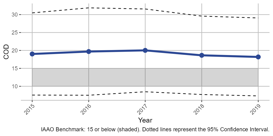
Price-Related Differential (PRD)
print(iaao_rslt[[3]])
#> [1] " In 2019, the PRD in  Cook County, Illinois, was 1.024 which <b>meets </b> the IAAO standard for vertical equity."
iaao_rslt[[4]]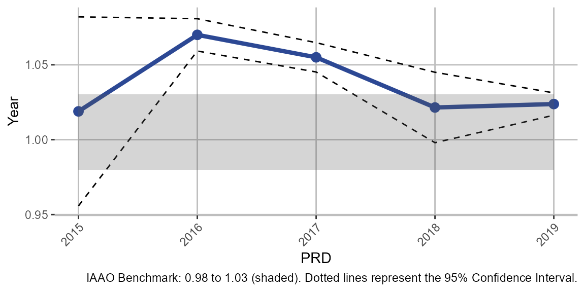
Coefficient of Price-Related Bias (PRB)
print(iaao_rslt[[5]])
#> [1] "In 2019, the PRB in Cook County, Illinois was 0.01 which indicates that sales ratios increase by 1.0% when home values double. This <b>meets </b>the IAAO standard."
iaao_rslt[[6]]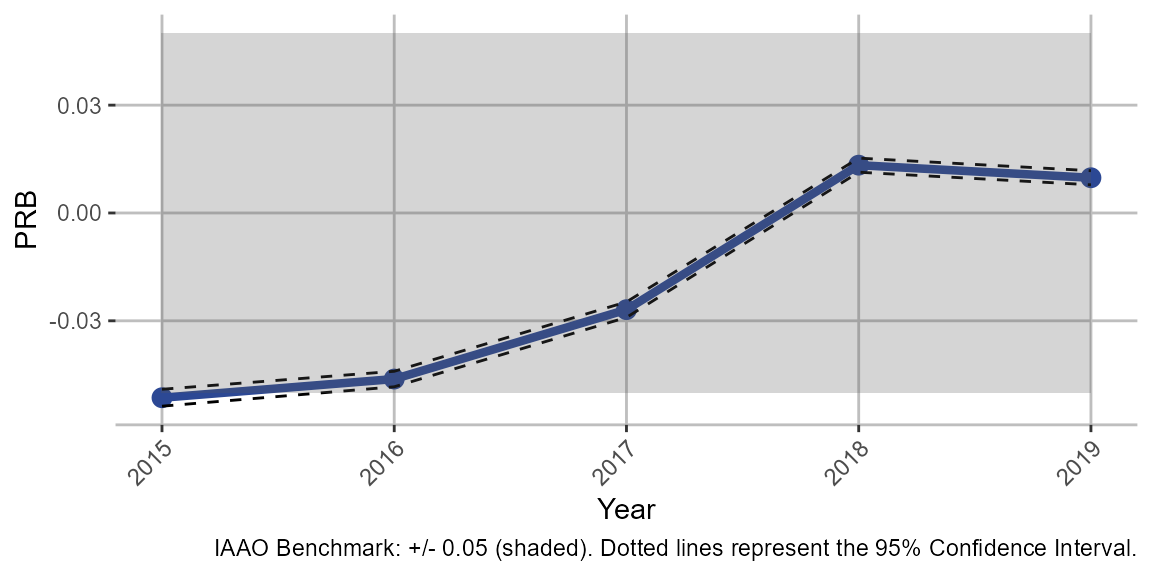
monte_carlo_graphs
m_rslts <- cmfproperty::monte_carlo_graphs(ratios)
gridExtra::grid.arrange(m_rslts[[1]],
                        m_rslts[[2]],
                        m_rslts[[3]],
                        m_rslts[[4]],
                        m_rslts[[5]],
                        m_rslts[[6]],
                        nrow = 3)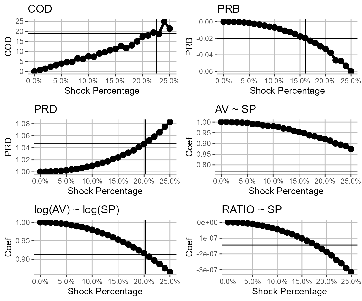
diagnostic_plots
plots <-
  diagnostic_plots(stats,
                   ratios,
                   min_reporting_yr = 2015,
                   max_reporting_yr = 2019)
plots[[1]]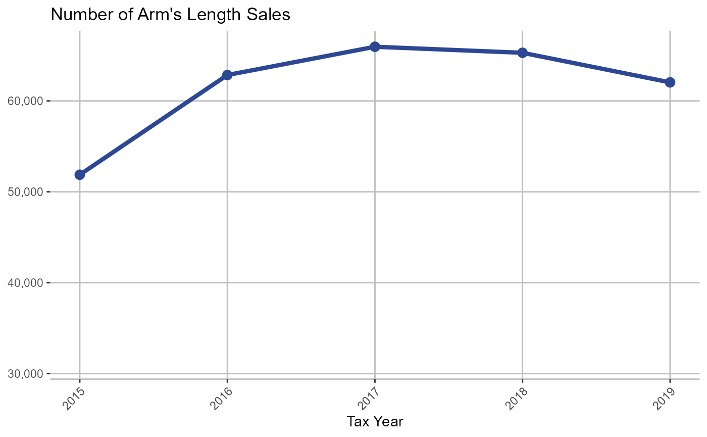
plots[[2]]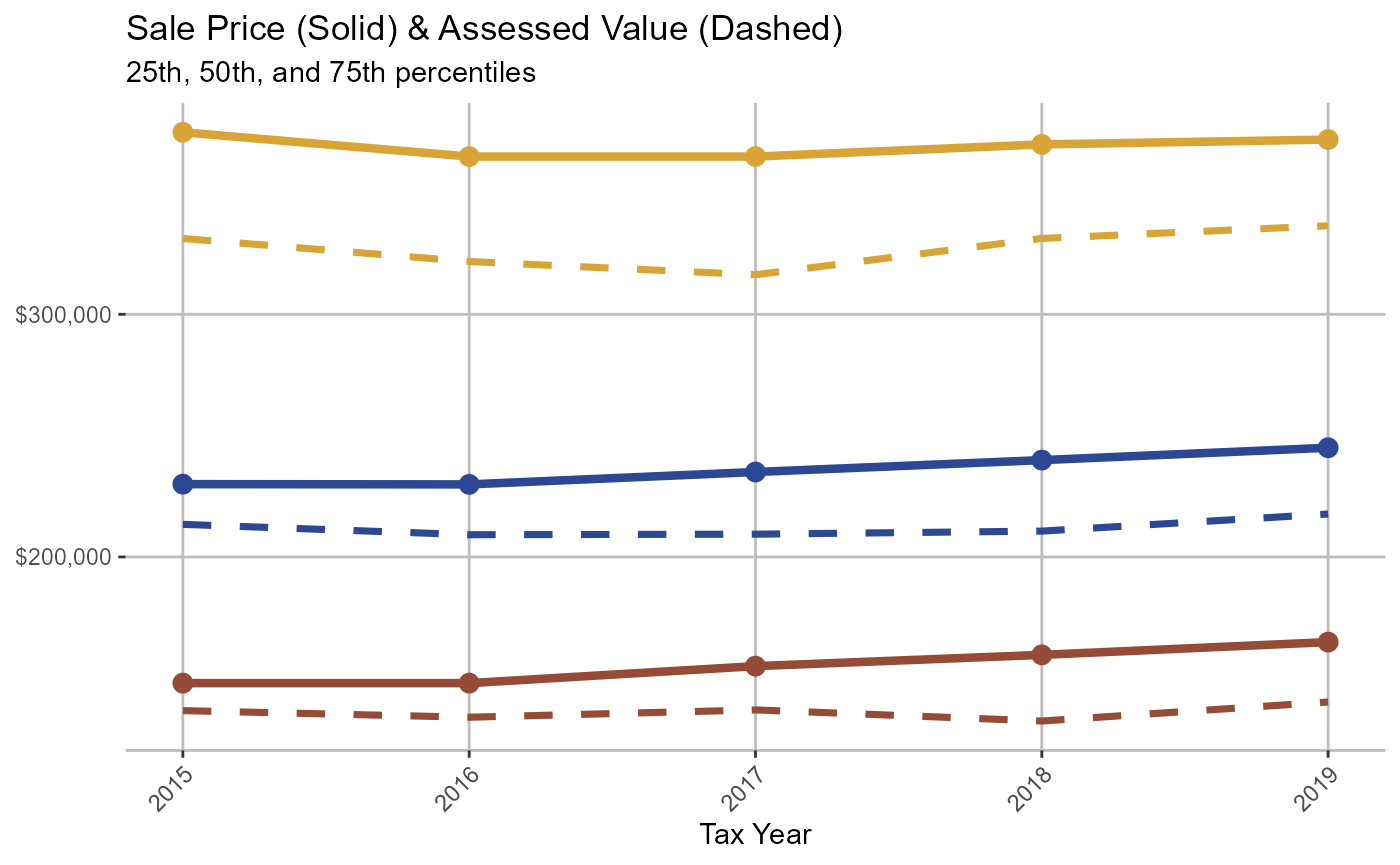
plots[[3]]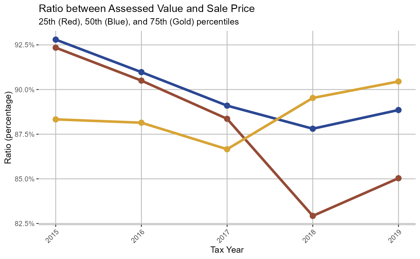
plots[[4]]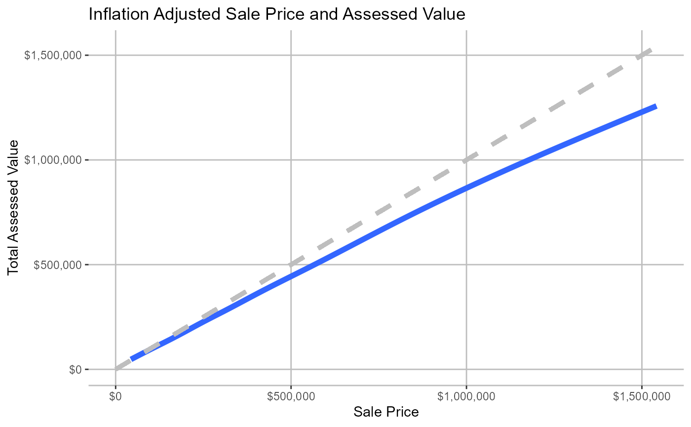
plots[[5]]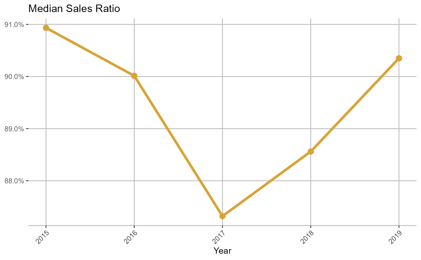
gridExtra::grid.arrange(plots[[6]],
                        plots[[7]],
                        plots[[8]],
                        plots[[9]],
                        ncol = 2,
                        nrow = 2)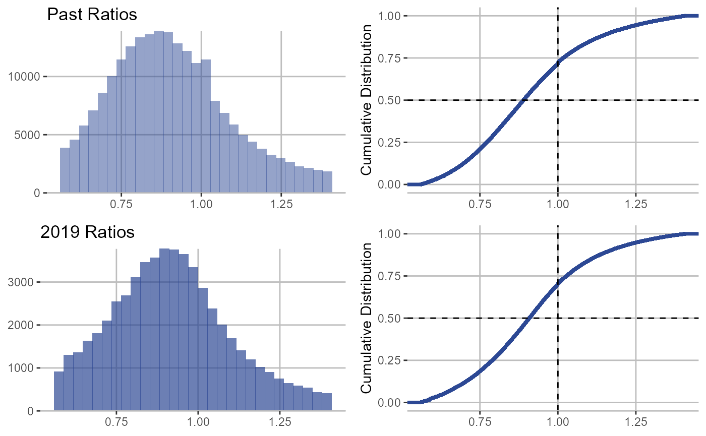
binned_scatter
binned <-
  cmfproperty::binned_scatter(
    ratios,
    min_reporting_yr = 2015,
    max_reporting_yr = 2019,
    jurisdiction_name = "Cook County, IL"
  )

print(binned[[1]])
#> [1] "In 2019, the most expensive homes (the top decile) were assessed at 87.1% of their value and the least expensive homes (the bottom decile) were assessed at 102.0%. In other words, the least expensive homes were assessed at <b>1.17 times</b> the rate applied to the most expensive homes. Across our sample from 2015 to 2019, the most expensive homes were assessed at 83.4% of their value and the least expensive homes were assessed at 109.4%, which is <b>1.31 times</b> the rate applied to the most expensive homes."
binned[[2]]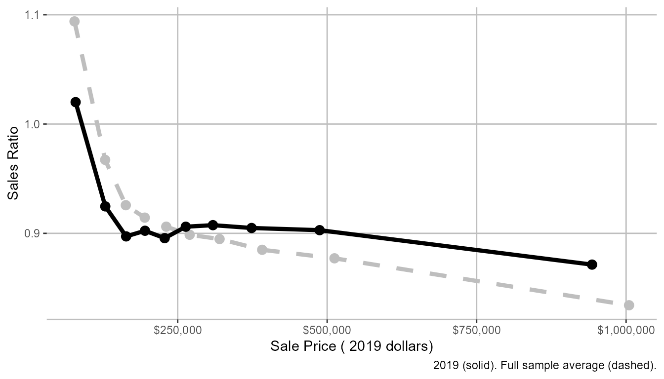
pct_over_under
pct_over <-
cmfproperty::pct_over_under(
ratios,
min_reporting_yr = 2015,
max_reporting_yr = 2019,
jurisdiction_name = "Cook County, IL"
)
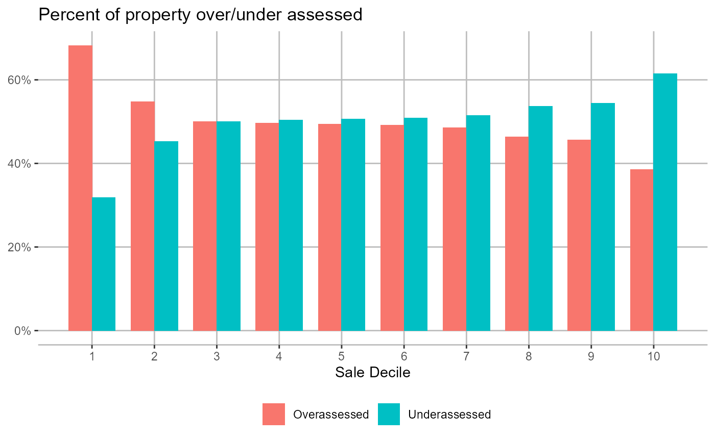
print(pct_over[[1]])
#> [1] "In Cook County, IL, <b>68%</b> of the lowest value homes are overassessed and <b>39%</b> of the highest value homes are overassessed."
pct_over[[2]]